Mathematics — Part 1
One of the greatest motivating forces for Donald Knuth when he began developing the original TeX system was to create something that allowed simple construction of mathematical formulae, whilst looking professional when printed. The fact that he succeeded was most probably why Tex (and later on, LaTeX) became so popular within the scientific community. Regardless of the history, typesetting mathematics is one of LaTeX's greatest strengths. However, it is also a large topic due to the existence of so much mathematical notation. So, this will be part one - getting to know the basics.
Maths environments
LaTeX needs to know beforehand that the subsequent text does in fact contain mathematical elements. This is because LaTeX typesets maths notation differently than normal text. Therefore, special environments have been declared for this purpose. They can be distinguished into two categories depending on how they are presented:
- text - text formulae are displayed inline, that is, within the body of text were it is declared. e.g., I can say that a + a = 2a within this sentence.
- displayed - displayed formulae are separate from the main text.
As maths require special environments, there are naturally the appropriate environment names you can use in the standard way. Unlike most other environments however, there are some handy shorthands to declaring your formulae. The following table summarises them:
| Type | Environment | LaTeX shorthand | Tex shorthand |
|---|---|---|---|
| Text | \begin{math}...\end{math} | \(...\) | $...$ |
| Displayed | \begin{displaymath}...\end{displaymath} | \[...\] | $$...$$ |
Additionally, there is second possible environment for the displayed type of formulae: equation. The difference between this and displaymath is that equation also adds sequential equation numbers by the side. See mathenv.pdf for an illustration of how the various basic environments are used.
Symbols
Mathematics has lots and lots of symbols! If there is one aspect of maths that is difficult in LaTeX it is trying to remember how to produce them. There are of course a set of symbols that can be accessed directly from the keyboard:
+ - = ! / ( ) [ ] < > | ' :
Beyond those listed above, distinct commands must be issued in order to display the desired symbols. And there are a lot! Greek letters, set and relations symbols, arrows, binary operators, etc. Too many to remember, and in fact, they would overwhelm this tutorial if I tried to list them all. Therefore, for a complete reference document, try symbols.pdf. We will of course see some of these symbols used throughout the tutorial.
Fractions
To create a fraction, you must use the \frac{numerator}{denominator} command. (For those who need their memories refreshed, that's the top and bottom respectively!) You can also embed fractions within fractions, as shown in the examples below:
| \frac{x+y}{y-z} |  |
| \frac{\frac{1}{x}+\frac{1}{y}}{y-z} |  |
Powers and indices
Powers and indices are mathematically equivalent to superscripts and subscripts in normal text mode. The carat (^) character is used to raise something, and the underscore (_) is for lowering. How to use them is best shown by example:
| Power | x^n |  |
| x^{2n} |  |
|
| Index | n_i |  |
| n_{ij} |  |
Note: if more than one character is to be raised (or lowered) then you must group them using the curly braces ( { } ).
Also, if you need to assign both a power and an index to the same entity, then that is achieved like this: x^{2i}_{3j} (or x_{3j}^{2i}, order is not significant).
Roots
Typically, for the majority of times, you are after the square root, which is done easily using the following command: \sqrt{x}. However, this can be generalised to produce a root of any magnitude:
| \sqrt[n]{arg} | 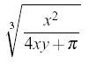 |
LaTeX will automatically ensure that the size of the root notation adjusts to the size of the contents.
The n is optional, and without it will output a square root. Also, regardless of the size of root you're after, e.g., n=3, you still use the \sqrt command.
Brackets
The use of brackets soon becomes important when dealing with anything but the most trivial equations. Without them, formulae can become ambiguous. Also, special types of mathematical structures, such as matrices typically rely on brackets to enclose them.
You may recall that you already have the ( ) [ ] symbols at your disposal, which should be more than adequate for most peoples' needs. So why the need for a dedicated section? Well, I think that can be shown by example:
| $$(\frac{x^2}{y^3})$$ |  |
| $$\left(\frac{x^2}{y^3}\right)$$ |  |
The first example shows what would happen if you used the standard bracket characters. As you can see, they would be fine for an equation a simple equation that remained on a single line (e.g., (3 + 2) x (10-3) = 35) but not for equations that have greater vertical size, such as those using fractions. The second example illustrates the LaTeX way of coping with this problem.
The \left... and \right... commands provide the means for automatic sizing of brackets. You must enclose the expression that you want in brackets with these commands. The dots after the command should be replaced with one of the characters depending on the style of bracket you want.
There are in fact many more possible symbols that can be used, but are somewhat uncommon. Please check out table 5 from the symbols reference (symbols.pdf) for the rest.
Matrices
LaTeX doesn't have a specific matrix command to use. It instead has a slightly more generalised environment called array. The array environment is basically equivalent to the table environment (see Tables tutorial to refresh your memory on table syntax.) Arrays are very flexible, and can be used for many purposes, but we shall focus on matrices. You can use the array to arrange and align your data as you want, and then enclose it with appropriate left and right brackets, and this will give you your matrix. For a simple 2x2 matrix:
$$ \left[
  \begin{array}{ c c }
     1 & 2 \\
     3 & 4
  \end{array} \right]
$$
|

|
Useful resources: symbols.pdf