Mathematics — Part 2
This tutorial builds on the basic foundations presented in the previous tutorial. If you often include a lot of maths in your documents, then you will probably find that you wish to have slightly more control over presentation issues. Some of the topics covered make writing equations more complex - but who said typesetting mathematics was easy?!
Adding text to equations
I doubt it will be every day that you will need to include some text within an equation. However, sometimes it needs to be done. Just sticking the text straight in the maths environment won't give you the results you want. For example:
\begin{equation}
  50 apples \times 100 apples = lots of apples
\end{equation}
|
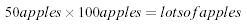 |
There are two noticeable problems. Firstly, there are no spaces between numbers and text, nor spaces between multiple words. Secondly, the words don't look quite right --- the letters are more spaced out than normal. Both issues are simply artifacts of the maths mode, in that it doesn't expect to see words. Any spaces that you type in maths mode are ignored and LaTeX spaces elements according to its own rules. It is assumed that any characters represent variable names. To emphasise that each symbol is an individual, they are not positioned as closely together as with normal text.
There are a number of ways that text can be added properly. The typical way is to wrap the text with the \mbox{...} command. This command hasn't been introduced before, however, it's job is basically to create a text box just width enough to contain the supplied text. Text within this box cannot be broken across lines. Let's see what happens when the above equation code is adapted:

The text looks better. However, there are no gaps between the numbers and the words. Unfortunately, you are required to explicitly add these. There are many ways to add spaces between maths elements, however, for the sake of simplicity, I find it easier, in this instance at least, just to literally add the space character in the affected \mbox(s) itself (just before the text.)
\begin{equation}
  50 \mbox{ apples} \times 100 \mbox{ apples} =
  \mbox{lots of apples}
\end{equation}
|
 |
Formatted text
Using the \mbox is fine and gets the basic result. Yet, there is an alternative that offers a little more flexibility. You may recall from the Formatting Tutorial, the introduction of font formatting commands, such as \textrm, \textit, \textbf, etc. These commands format the argument accordingly, e.g., \textbf{bold text} gives bold text. These commands are equally valid within a maths environment to include text. The added benefit here is that you can have better control over the font formatting, rather than the standard text achieved with \mbox.
\begin{equation}
  50 \textrm{ apples} \times 100 \textbf{ apples} =
  \textit{lots of apples}
\end{equation}
|
 |
However, as is the case with LaTeX, there is more than one way to skin a cat! There are a set of formatting commands very similar to the font formatting ones just used, except they are aimed specifically for text in maths mode. So why bother showing you \textrm and co if there are equivalents for maths? Well, that's because they are subtly different. The maths formatting commands are:
| Command | Format | Example |
|---|---|---|
| \mathrm{...} | Roman |  |
| \mathit{...} | Italic |  |
| \mathbf{...} | Bold |  |
| \mathsf{...} | Sans serif |  |
| \mathtt{...} | Typewriter |  |
| \mathcal{...} | Calligraphy |  |
The maths formatting commands can be wrapped around the entire equation, and not just on the textual elements: they only format letters, numbers, and uppercase Greek, and the rest of the maths syntax is ignored. So, generally, it is better to use the specific maths commands if required. Note that the calligraphy example gives rather strange output. This is because for letters, it requires upper case characters. The reminding letters are mapped to special symbols.
Changing text size of equations
Probably a rare event, but there may be a time when you would prefer to
have some control of the size. For example, using text-mode maths, by
default a simple fraction will look like this:  where as
you may prefer to have it displayed larger, like when in display mode,
but still keeping it inline, like this:
where as
you may prefer to have it displayed larger, like when in display mode,
but still keeping it inline, like this:  .
.
A simple approach is to utilise the predefined sizes for maths elements:
| \displaystyle | Size for equations in display mode |
| \textstyle | Size for equations in text mode |
| \scriptstyle | Size for first sub/superscripts |
| \scriptscriptstyle | Size for subsequent sub/superscripts |
A classic example to see this in use is typesetting continued fractions. The following code provides an example.
\begin{equation}
  x = a_0 + \frac{1}{a_1 + \frac{1}{a_2 + \frac{1}{a_3 + a_4}}}
\end{equation}
|
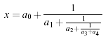 |
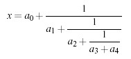
As you can see, as the fractions continue, they get smaller (although they will not get any smaller as in this example, they have reached the \srciptscriptstyle limit. If you wanted to keep the size consistent, you could declare each fraction to use the display style instead, e.g.,
\begin{equation}
  x = a_0 + \frac{1}{\displaystyle a_1
          + \frac{1}{\displaystyle a_2
          + \frac{1}{\displaystyle a_3 + a_4}}}
\end{equation}
|
 |
Another approach is to use the \DeclareMathSizes command to select your preferred sizes. You can only define sizes for \displaystyle}, \textstyle, etc. One potential downside is that this command sets the global maths sizes, as it can only be used in the document preamble.
However, it's fairly easy to use: \DeclareMathSizes{ds}{ts}{ss}{sss}, where ds is the display size, ts is the text size, etc. The values you input are assumed to be point (pt) size. In the example document (mathsize2.pdf), the math sizes have been made much larger than necessary to illustrate that the changes have taken place.
NB the changes only take place if the value in the first argument matches the current document text size. It is therefore common to see a set of declarations in the preamble, in the event of the main font being changed. E.g.,
\DeclareMathSizes{10}{18}{12}{8}   % For size 10 text
\DeclareMathSizes{11}{19}{13}{9}   % For size 11 text
\DeclareMathSizes{12}{20}{14}{10}  % For size 12 text
Multi-lined equations (eqnarray environment)
Imagine that you have an equation that you want to manipulate, for example, to simplify it. Often this is done over a number of steps to help the reader understand how to get from the original equation to the final result. This should be a relatively simple task, but as we shall see, the skills for displaying mathematics from the previous tutorial are not adequate. Using what we know so far:
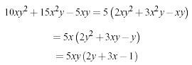
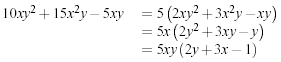
This clearly looks rather ugly. One way to the various elements neatly aligned is to use a table, and place equations inline. Let's have a go:
\begin{tabular}{ r l }
\(10xy^2+15x^2y-5xy\) & \(= 5\left(2xy^2+3x^2y-xy\right)\) \\
 & \(= 5x\left(2y^2+3xy-y\right)\) \\
 & \(= 5xy\left(2y+3x-1\right)\)
 \end{tabular}
|
 |
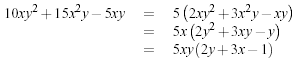
That doesn't look too bad. Perhaps the extra space between the equation on the left and the equals sign being larger than the gap on the right doesn't look perfect. That could be rectified by adding an extra column and putting the equals sign in the central one:
\begin{tabular}{ r c l }
  \(10xy^2+15x^2y-5xy\) & \(=\) & \(5\left(2xy^2+3x^2y-xy\right)\) \\
   & \(=\) & \(5x\left(2y^2+3xy-y\right)\) \\
   & \(=\) & \(5xy\left(2y+3x-1\right)\)
\end{tabular}
|
 |
Looking better. Another issue is that the vertical space between the rows makes makes the equations on the right-hand side look a little crowded. It would be nice to add a little space --- make the rows in the table a little taller. (You need to add \usepackage{array} to your preamble for this to work.)
% add some extra height. Needs the array package. See preamble.
\setlength{\extrarowheight}{0.3cm}
However, by this stage, we've had to do quite a bit of extra leg work, and there is still one important disadvantage at the end of it. You can't add equation numbers. Because once you are within the tabular environment, you can only use the inline type of maths display. For equation numbers, you need to use the display mode equation package, but you can't in this instance. This is where eqnarray becomes extremely useful.
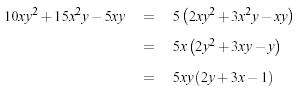
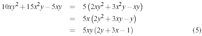
eqnarray, as the name suggests borrows from the array} package which is basically a simplified tabular environment. The array package was introduced in the Mathematics 1 tutorial for producing matrices. Here is how to use eqnarray for this example:
\begin{eqnarray}
  10xy^2+15x^2y-5xy & = & 5\left(2xy^2+3x^2y-xy\right) \\
   & = & 5x\left(2y^2+3xy-y\right) \\
   & = & 5xy\left(2y+3x-1\right)
\end{eqnarray}
|
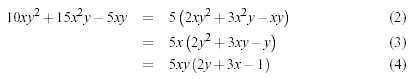 |
As you can see, everything is laid out nicely and as expected. Well, except that each row within the array has been assigned its own equation number. Whilst this feature is useful in some instances, it is not required here --- just the one number will do! To suppress equation numbers for a given row, add a \nonumber command just before the end of row command (\\).
\begin{eqnarray}
  10xy^2+15x^2y-5xy & = & 5\left(2xy^2+3x^2y-xy\right) \nonumber \\
   & = & 5x\left(2y^2+3xy-y\right) \nonumber \\
   & = & 5xy\left(2y+3x-1\right)
\end{eqnarray}
|
|
If you don't care for equation numbers at all, then rather than adding \nonumber to every row, use the starred version of the environment, i.e., \begin{eqnarray*} ... \end{eqnarray*}.
NB There is a limit of 3 columns in the eqnarray environment. If you need anymore flexibility, you are best advised to seek the AMS Maths packages.
Breaking up long equations
Let us first see an example of a long equation. (Note, when you view the example document for this topic, you will see that this equation is in fact wider than the text width. It's not as obvious on this webpage!)
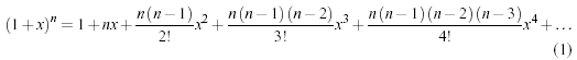
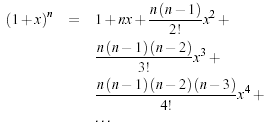
LaTeX doesn't break long equations to make them fit within the margins as it does with normal text. It is therefore up to you to format the equation appropriately (if they overrun the margin.) This typically requires some creative use of an eqnarray to get elements shifted to a new line and to align nicely. E.g.,
\begin{eqnarray*}
  \left(1+x\right)^n & = & 1 + nx + \frac{n\left(n-1\right)}{2!}x^2 \\
  & & + \frac{n\left(n-1\right)\left(n-2\right)}{3!}x^3 \\
  & & + \frac{n\left(n-1\right)\left(n-2\right)\left(n-3\right)}{4!}x^4 \\
  & & + \ldots
\end{eqnarray*}
|
 |
It may just be that I'm more sensitive to these kind of things, but you may notice that from the 2nd line onwards, the space between the initial plus sign and the subsequent fraction is (slightly) smaller than normal. (Observe the first line, for example.) This is due to the fact that LaTeX deals with the + and - signs in two possible ways. The most common is as a binary operator. When two maths elements appear either side of the sign, it is assumed to be a binary operator, and as such, allocates some space either side of the sign. The alternative way is a sign designation. This is when you state whether a mathematical quantity is either positive or negative. This is common for the latter, as in maths, such elements are assumed to be positive unless a - is prefixed to it. In this instance, you want the sign to appear close to the appropriate element to show their association. It is this interpretation that LaTeX has opted for in the above example.
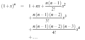
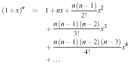
To add the correct amount of space, you can add an invisible character using {}, as illustrated here:
\begin{eqnarray*}
  \left(1+x\right)^n & = & 1 + nx + \frac{n\left(n-1\right)}{2!}x^2 \\
  & & {} + \frac{n\left(n-1\right)\left(n-2\right)}{3!}x^3 \\
  & & {} + \frac{n\left(n-1\right)\left(n-2\right)\left(n-3\right)}{4!}x^4 \\
  & & {} + \ldots
\end{eqnarray*}
|
|
Alternatively, you could avoid this issue altogether by leaving the + at the end of the previous line rather at the beginning of the current line:
There is another convention of writing long equations that LaTeX supports. This is the way I see long equations typeset in books and articles, and admittedly is my preferred way of displaying them. Sticking with the eqnarray approach, using the \lefteqn{...} command around the content before the = sign gives the following result:
\begin{eqnarray*}
  \lefteqn{\left(1+x\right)^n = } \\
  & & 1 + nx + \frac{n\left(n-1\right)}{2!}x^2 + \\
  & & \frac{n\left(n-1\right)\left(n-2\right)}{3!}x^3 + \\
  & & \frac{n\left(n-1\right)\left(n-2\right)\left(n-3\right)}{4!}x^4 + \\
  & & \ldots
\end{eqnarray*}
|
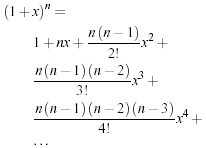 |
Notice that the first line of the eqnarray contains the \lefteqn only. And within this command, there are no column separators (&). The reason this command displays things as it does is because the \lefteqn prints the argument, however, tells LaTeX that the width is zero. This results in the first column being empty, with the exception of the inter-column space, which is what gives the subsequent lines their indentation.
Controlling horizontal spacing
LaTeX is obviously pretty good at typesetting maths --- it was one of the chief aims of the core Tex system that LaTeX extends. However, it can't always be relied upon to accurately interpret formulae in the way you did. It has to make certain assumptions when there are ambiguous expressions. The result tends to be slightly incorrect horizontal spacing. In these events, the output is still satisfactory, yet, any perfectionists will no doubt wish to fine-tune their formulae to ensure spacing is correct. These are generally very subtle adjustments.
There are other occasions where LaTeX has done its job correctly, but you just want to add some space, maybe to add a comment of some kind. For example, in the following equation, it is preferable to ensure there is a decent amount of space between the maths and the text.
\[f(n) = \left\{
\begin{array}{l l}
  n/2 & \quad \mbox{if $n$ is even}\\
  -(n+1)/2 & \quad \mbox{if $n$ is odd}\\ \end{array} \right. \]
|
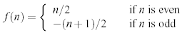 |
LaTeX has defined two commands that can be used anywhere in documents (not just maths) to insert some horizontal space. They are \quad and \qquad
A \quad is a space equal to the current font size. So, if you are using an 11pt font, then the space provided by \quad will also be 11pt (horizontally, of course.) The \qquad gives twice that amount. As you can see from the code from the above example, \quads were used to add some separation between the maths and the text.
OK, so back to the fine tuning as mentioned at the beginning of the document. A good example would be displaying the simple equation for the indefinite integral of y with respect to x:

If you were to try this, you may write:
\[ \int y \mathrm{d}x \]
|

|
However, this doesn't give the correct result. LaTeX doesn't respect the whitespace left in the code to signify that the y and the dx are independent entities. Instead, it lumps them altogether. A \quad would clearly be overkill is this situation --- what is needed are some small spaces to be utilised in this type of instance, and that's what LaTeX provides:
| Command | Description | Size |
|---|---|---|
| \, | small space | 3/18 of a quad |
| \: | medium space | 4/18 of a quad |
| \; | large space | 5/18 of a quad |
| \! | negative space | -3/18 of a quad |
NB you can use more than one command in a sequence to achieve a greater space if necessary.
So, to rectify the current problem:
| \int y\, \mathrm{d}x |  |
| \int y\: \mathrm{d}x |  |
| \int y\; \mathrm{d}x |  |
The negative space may seem like an odd thing to use, however, it wouldn't be there if it didn't have some use! Take the following example:
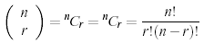
The matrix-like expression for representing binomial coefficients is too padded. There is too much space between the brackets and the actual contents within. This can easily be corrected by adding a few negative spaces after the left bracket and before the right bracket.
\[\left(\!\!\!
  \begin{array}{c}
    n \\
    r
  \end{array}
  \!\!\!\right) = {^n}C_r = \frac{n!}{r!(n-r)!}
\]
|
 |
Summary
As you can begin to see, typesetting maths can be tricky at times. However, because LaTeX provides so much control, you can get professional quality mathematics typesetting for relatively little effort (once you've had a bit of practise, of course!). It would be possible to keep going and going with maths topics because it seems potentially limitless. However, with these two tutorials, you should be able to get along sufficiently.
Useful resources: User's Guide for the amsmath Package [pdf]